David Silver 교수님의 강의 내용을 정리하고자 한다(링크).
0. Introduction
RL은 아래와 같이 굉장히 큰 크기의 문제들을 풀 수 있다.
- Backgammon: $10^{20}$ states
- Computer Go: $10^{170}$ states
- Helicopter: continuous state space
5장에서 배웠던 model-free 환경에서의 prediction, control 문제들에 대해 scale up 할 수 있는 방법을 이번 장에서 배울 것이다.
*So far we, we have represented valu function by a lookup table.
- Every state $s$ has an entry $V(s)$
- Or every state-action pair $s,a$ has an entry $Q(s,a)$
*Problem with large MDPs:
- There are too many states and/or actions to store in memory
- Too slow to learn the value of each state individually
*Solution for large MDPs:
- Estimate value function with parametric function approximation
$$\begin{array}{rcl}
\hat{v}(s, \mathrm{w}) & \approx & v_{\pi}(s) \\
\hat{q}(s, a,\mathrm{w}) & \approx & q_{\pi}(s,a)
\end{array}$$
- Generalize from seen states to unseen states
- Update parameter $\mathrm{w}$ using MC or TD learning
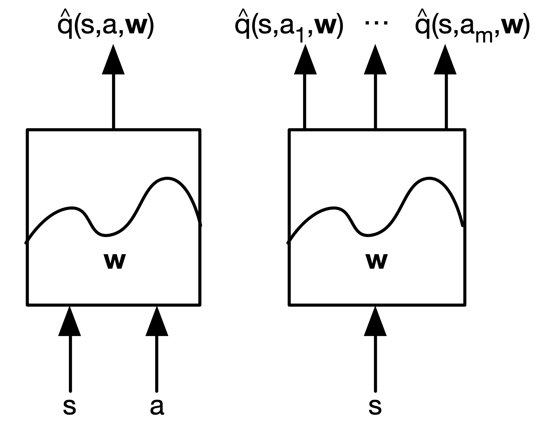
[Types of Value Function Approximation]
| value approx. | action-value approx. |
 |
 |
Function approximation에는 다양한 방법이 있지만 본 장에서는 differentiable하고, non-stationary(time-dependent) & non-iid 데이터에 적합한 linear combinations of feature, neural network만 고려한다.
1. Incremental Methods
(1) Gradient Descent
- Let $J(\mathrm{w})$ be a differentiable function of parameter vector $\mathrm{w}$
- Define the gradient of $J(\mathrm{w})$ to be
$$\nabla_{\mathrm{w}} J(\mathrm{w}) = \begin{pmatrix}
\frac{\partial J(\mathrm{w})}{\partial \mathrm{w}_{1}} \\
\vdots \\
\frac{\partial J(\mathrm{w})}{\partial \mathrm{w}_{n}}
\end{pmatrix}$$
- To find a local minimum of $J(\mathrm{w})$, adjust $\mathrm{w}$ in direction of -ve gredient($\alpha$: step-size parameter)
$$\Delta \mathrm{w} = - \frac{1}{2}\alpha \nabla_{\mathrm{w}} J(\mathrm{w}) $$
[Value Function Approximation by Stochastic Gradient Descent]
- Goal: find parameter vector $\color{red}\mathrm{w}$ minimizing mean-squared error between approximate value fn $\color{red}\hat{v}(s, \mathrm{w})$ and true value fn $\color{red}v_{\pi}(s)$
$$J(\mathrm{w})=\mathbb{E}_{\pi}[( v_{\pi}(S)-\hat{v}(S,\mathrm{w}))^{2}]$$
- Gradient descent finds a local minimum
$$\begin{array}{rcl}
\Delta \mathrm{w} & = & - \frac{1}{2}\alpha \nabla_{\mathrm{w}} J(\mathrm{w})\\
& = & \alpha \mathbb{E}_{\pi}[( v_{\pi}(S)-\hat{v}(S,\mathrm{w}))\nabla_{\mathrm{w}}\hat{v}(S,\mathrm{w}) ] \\
& & v_{\pi}(S)-\hat{v}(S,\mathrm{w}): \text{error in each step}
\end{array}$$
- Stochastic gradient descent samples the gradient
$$\Delta \mathrm{w} = \alpha(v_{\pi}(S)-\hat{v}(S,\mathrm{w}))\nabla_{\mathrm{w}}\hat{v}(S,\mathrm{w})$$
Expected update is equal to full gradient update
(2) Linear Function Approximation
*Feature Vectors: represent state by a feature vector(e.g. distance of robot from landmarks, trends in the stock market..)
$$\mathrm{x}(S) = \begin{pmatrix}
\mathrm{x}_{1}(S) \\
\vdots \\
\mathrm{x}_{n}(S)
\end{pmatrix}$$
[Linear Function Approximation]
- Represent value function by a linear combination of feature
$$\hat(v)(S,\mathrm{w}) = \mathrm{x}(S)^{T}\mathrm{w} = \sum_{j=1}^{n}\mathrm{x}_{j}(S)\mathrm{w}_{j}$$
- Objective function is quadratic in parameters $\mathrm{w}$
$$J(\mathrm{w}) = \mathbb{E}_{\pi}[(v_{\pi}(S)-\mathrm{x}(S)^{T}\mathrm{w})^{2}]$$
- Stochastic gradient descent converges on global optimum
- Update rule is particularly simple: $\text{Update = step-size} \times \text{prediction error} \times \text{feature value}$
$$\begin{array}{rcl}
\nabla _{\mathrm{w}}\hat{v}(S,\mathrm{w}) &=& \mathrm{x}(S) \\
\Delta_{\mathrm{w}}\mathrm{w} & = & \alpha(v_{\pi}(S)-\hat{v}(S,\mathrm{w}))\mathrm{x}(S)
\end{array}$$
*Table Lookup Features
- Table lookup is a special case of linear value function approximation
- Using table lookup features
$$\mathrm{x}^{\text{table}}(S) = \begin{pmatrix}
\textbf{1}(S=s_{1}) \\
\vdots \\
\textbf{1}(S=s_{n})
\end{pmatrix}$$
- Parameter vector $\mathrm{w}$ gives value of each individual state
$$\hat{v}(S,\mathrm{w}) = \begin{pmatrix}
\textbf{1}(S=s_{1}) \\
\vdots \\
\textbf{1}(S=s_{n})
\end{pmatrix} \cdot\begin{pmatrix}
\mathrm{w}_{1} \\
\vdots \\
\mathrm{w}_{n}
\end{pmatrix}$$
(3) Incremental Prediction Algorithms
- Have assumed true value function $v_{\pi}(s)$ given by supervisor
- But in RL there is no supervisor, only rewards
- In practice, we substitute a target for $\color{red}v_{\pi}(s)$:
- (★)For MC, the target is the return $\color{red}G_{t}$
$$\Delta\mathrm{w} = \alpha(\color{red} G_{t} \color{black} - \hat{v}(S_{t},\mathrm{w}))\nabla _{\mathrm{w}}\hat{v}(S,\mathrm{w})$$
- (★)For TD(0), the target is the TD target $\color{red}R_{t+1}+\gamma \hat{v}(S_{t+1},\mathrm{w})$
$$\Delta\mathrm{w} = \alpha(\color{red}R_{t+1}+\gamma\hat{v}(S_{t+1},\mathrm{w})\color{black}-\hat{v}(S,\mathrm{w}))\nabla_{\mathrm{w}}\hat{v}(S_{t},\mathrm{w})$$
- (★)For TD($\lambda$), the target is the $\lambda$-return $\color{red}G^{\lambda}_{t}$
$$\Delta \mathrm{w} = \alpha(\color{red}G^{\lambda}_{t}\color{black}-\hat{v}(S_{t},\mathrm{w}))\nabla_{\mathrm{w}}\hat{v}(S_{t},\mathrm{w})$$
[MC with Value Function Approximation]
- Return $G_{t}$ is an "unbiased", noisy sample of true value $v_{\pi}(S_{t})$
- Can therefore apply supervised learning to training data:
$$\left\langle S_{1},G_{1} \right\rangle,\left\langle S_{2},G_{2} \right\rangle.\dots,\left\langle S_{T},G_{T} \right\rangle$$
- For example, using linear Monte -Carlo policy evaluation,
$$\begin{array}{rcl}
\Delta\mathrm{w} & = & \alpha(\color{red}G_{t}\color{black}-\hat{v}(S_{t},\mathrm{w}))\nabla_{\mathrm{w}}\hat{v}(S_{t},\mathrm{w}) \\
& = & \alpha(\color{red}G_{t}\color{black}-\hat{v}(S_{t},\mathrm{w})) \mathrm{x}(S_{t})
\end{array}$$
- MC evaluation converges to a local optimum, even when using non-linear value function approximation
[TD Learning with Value Function Approximation]
- The TD target $R_{t+1}+\gamma \hat{v}(S_{t+1},\mathrm{w})$ is a "biased" sample of true value $v_{\pi}(S_{t})$
- Can still apply supervised learning to training data:
$$\left\langle S_{1},R_{2}+\gamma \hat{v}(S_{2},\mathrm{w}) \right\rangle,\left\langle S_{2},R_{3}+\gamma \hat{v}(S_{3},\mathrm{w}) \right\rangle.\dots,\left\langle S_{T-1},R_{T} \right\rangle$$
- For example, using linear TD(0))
$$\begin{array}{rcl}
\Delta\mathrm{w} & = & \alpha(\color{red}R+\gamma \hat{v}(S^{'},\mathrm{w})\color{black}-\hat{v}(S^{'},\mathrm{w}))\nabla_{\mathrm{w}}\hat{v}(S^{'},\mathrm{w}) \\
& = & \alpha\delta\mathrm{x}(S)
\end{array}$$
- Linear TD(0) converges (close) to global optimum
[TD($\lambda$) with Value Function Approximation]
- The $\lambda$-return $G_{t}^{\lambda}$ is also a "biased" sample of true value $v_{\pi}(S)$
- Can again apply supervised learning to training data:
$$\left\langle S_{1},G_{1}^{\lambda} \right\rangle,\left\langle S_{2},G_{2}^{\lambda} \right\rangle.\dots,\left\langle S_{T-1},G_{T-1}^{\lambda} \right\rangle$$
- Forward view linear TD($\lambda$)
$$\begin{array}{rcl}
\Delta\mathrm{w} & = & \alpha(\color{red}G_{t}^{\lambda}\color{black}-\hat{v}(S^{'}_{t},\mathrm{w}))\nabla_{\mathrm{w}}\hat{v}(S^{'}_{t},\mathrm{w}) \\
& = & \alpha(\color{red}G_{t}^{\lambda}\color{black}-\hat{v}(S^{'}_{t},\mathrm{w}))\mathrm{x}(S_{t})
\end{array}$$
- Backward view linear TD($\lambda$)
$$\begin{array}{rcl}
\delta_{t} &=& R_{t+1}+\gamma\hat{v}(S_{t+1},\mathrm{w})-\hat{v}(S_{t},\mathrm{w}) \\
E_{t} & = & \gamma\lambda E_{t+1}+\mathrm{x}(S_{t}) \\
\Delta\mathrm{w} & = & \alpha\delta_{t}E_{t}
\end{array}$$
- Foward view and backward view linear TD($\lambda$) are equivalent
(4) Incremental Control Algorithms
[Control with Value Function Approximation]

이전 부분은 value function approximation에 대한 내용이었고 이 부분은 action-value function approximation에 대한 내용이다.
[Action-Value Function Approximation]
- Approximate the action-value function
$$\hat{q}(S,A,\mathrm{w}) \approx q_{\pi}(S,A)$$
- Minimize mean-squared error between approximate action-value fn $\hat{q}(S,A,\mathrm{w})$ and true action-value fn $q_{\pi}(S,A)$
$$J(\mathrm{w}) = \mathbb{E}_{\pi}[(q_{\pi}(S,A)-\hat{q}(S,A,\mathrm{w}))^{2}]
\\
\hat{q}(S,A,\mathrm{w}) \approx q_{\pi}(S,A)$$
- Use SGD to find a local minimum
$$\begin{array}{rcl}
-\frac{1}{2}\nabla_{\mathrm{w}}J(\mathrm{w})&=& (q_{\pi}(S,A)-\hat{q}(S,A,\mathrm{w}))\nabla_{\mathrm{w}}\hat{q}(S,A,\mathrm{w}) \\
\Delta\mathrm{w} & = & \alpha(q_{\pi}(S,A)-\hat{q}(S,A,\mathrm{w}))\nabla_{\mathrm{w}}\hat{q}(S,A,\mathrm{w})
\end{array}$$
[Linear Action-Value Function Approximation]
- Represent state and action by a feature vector
$$\mathrm{x}(S,A) = \begin{pmatrix}
\mathrm{x}_{1}(S,A) \\
\vdots \\
\mathrm{x}_{n}(S,A)
\end{pmatrix}$$
- Represent action-value fn by linear combination of feature
$$\hat{q}(S,A,\mathrm{w}) = \mathrm{x}(S,A)^{T}\mathrm{w}=\sum_{j=1}^{n}\mathrm{x}_{j}(S,A)\mathrm{w}_{j}$$
- Stochastic gradient descent update
$$\begin{array}{rcl}
\nabla_{\mathrm{w}}\hat{q}(S,A,\mathrm{w}) & = & \mathrm{x}(S,A) \\
\Delta\mathrm{w} & = & \alpha(q_{\pi}(S,A)-\hat{q}(S,A,\mathrm{w}))\mathrm{x}(S,A)
\end{array}$$
[Incremental Control Algorithms]
- Like prediction, we must substitue a target for $\color{red}q_{\pi}(S,A)$
- (★)For MC, the target is the return $\color{red}G_{t}$
$$\Delta\mathrm{w} = \alpha(\color{red} G_{t} \color{black} - \hat{q}(S_{t},A_{t},\mathrm{w}))\nabla_{\mathrm{w}}\hat{q}(S_{t},A_{t},\mathrm{w})$$
- (★)For TD(0), the target is the TD target $\color{red}R_{t+1}+\gamma \hat{v}(S_{t+1},\mathrm{w})$
$$\Delta\mathrm{w} = \alpha(\color{red}R_{t+1}+\gamma\hat{q}(S_{t+1},A_{t+1},\mathrm{w})\color{black}-\hat{q}(S_{t},A_{t},\mathrm{w}))\nabla_{\mathrm{w}}\hat{q}(S_{t},A_{t},\mathrm{w})$$
- (★)For forward-view TD($\lambda$), target is the action-value $\lambda$-return
$$\Delta \mathrm{w} = \alpha(\color{red}q^{\lambda}_{t}\color{black}-\hat{q}(S_{t},A_{t},\mathrm{w}) )\nabla_{\mathrm{w}}\hat{q}(S_{t},A_{t},\mathrm{w}) $$
- For backward-view TD($\lambda$), equivalent update is
$$\begin{array}{rcl}
\delta_{t} &=& R_{t+1}+\gamma\hat{q}(S_{t},A_{t},\mathrm{w})-\hat{q}(S_{t},A_{t},\mathrm{w}) \\
E_{t} & = & \gamma\lambda E_{t+1}+\nabla_{\mathrm{w}}\hat{q}(S_{t},A_{t},\mathrm{w}) \\
\Delta\mathrm{w} & = & \alpha\delta_{t}E_{t}
\end{array}
$$
(5) Convergence

- Convergence of Prediction Algorithms

[Gradient Temporal-Difference Learning]
- TD does not follow the gradient of any objective function
- This is why TD can diverge when off-policy or using non-linear function approximation
- Gradient TD follows true gradient of projected Bellman error

*Convergence of Control Algorithms

2. Batch Methods
Gradient descent is simple and appealing. But it is not sample efficient(위 방법들은 하나의 sample로 값을 update하고 이후엔 사용하지 않음). Batch methods seek to find the best fitting value function, give the agent's experience('training data')
(1) Least Squares Prediction
[Least Squares Predictions]
- Given value function approximation $\hat{v}(s, \mathrm{w}) \approx v_{\pi}(s)$
- and experience $\mathcal{D}$ consisting of $\left\langle \text{state, value} \right\rangle$ paris
$$\mathcal{D} = \left\{ \left\langle s_{1}, v_{1}^{\pi} \right\rangle, \left\langle s_{2}, v_{2}^{\pi} \right\rangle, \dots, \left\langle s_{T}, v_{T}^{\pi} \right\rangle \right\}$$
- Which parameters $\mathrm{w}$ gives the best fitting value function $\hat{v}(s, \mathrm{w})$?
- Least Squares algorithms find parameter vector $\mathrm{w}$ minimizing sum-squared error between $\hat{v}(s_{t}, \mathrm{w})$ and target values $v_{t}^{\pi}$
$$\begin{array}{rcl}
LS(\mathrm{w}) & = & \sum_{t=1}^{T} (v_{t}^{\pi}- \hat{v}(s_{t}, \mathrm{w}))^{2} \\
& = & \mathbb{E}_{\mathcal{D}}\left[ (v_{t}^{\pi}- \hat{v}(s_{t}, \mathrm{w}))^{2} \right] \\
& & \mathbb{E}: \text{empirical distribution}
\end{array}$$
*Stochastic Gradient Descent with Experience Replay
- Experience Replay: data를 캐싱해두고 반복적으로 사용
- Given experience consisting of $\left\langle \text{state, value} \right\rangle$ paris
$$\mathcal{D} = \left\{ \left\langle s_{1}, v_{1}^{\pi} \right\rangle, \left\langle s_{2}, v_{2}^{\pi} \right\rangle, \dots, \left\langle s_{T}, v_{T}^{\pi} \right\rangle \right\}$$
Repeat:
- Sample state, value from experience
$$\left\langle s, v^{\pi} \right\rangle \sim\mathcal{D} $$
- Apply stochastic gradient descent update
$$\Delta \mathrm{w} = \alpha(v^{\pi}- \hat{v}(s, \mathrm{w}))\nabla_{\mathrm{w}}\hat{v}(s, \mathrm{w})$$
Converges to least squares solution
$$\mathrm{w}^{\pi} = \underset{\mathrm{w}}{\text{argmin}} \ LS(\mathrm{w})$$
*Experience Replay in Deep Q-Networks(DQN)
DQN uses experience replay(function approx. about Q) and fixed Q-targets(off-policy)
- Take action $a_{t}$ according to $\epsilon$-greedy policy
- Store transition $(s_{t}, a_{t}, r_{t+1}, s_{t+1})$ in replay memory $\mathcal{D}$
- Sample random mini-batch of transitions $(s,a,r,s^{'})$ from $\mathcal{D}$
- Compute Q-learning targets w.r.t. old, fixed parameters $\mathrm{w}^{-}$
- Optimize MSE between Q-network and Q-learning targets
$$\mathcal{L}_{i}(\mathrm{w}_{i}) = \mathbb{E}_{s,a,r,s^{'}\sim \mathcal{D}_{i} }\left[ (r+\gamma \underset{a^{'}}{\text{max}} \ Q(s^{'},a^{'};\mathrm{w}_{i}^{-})-Q(s,a;\mathrm{w}_{i}) )^{2} \right]$$
*How much does DQN help?

[Linear Least Squares Predictions Algorithms]
Experience replay finds least squares solution but it may take many iterations. Using linear value function approximation, $\hat{v}(s,\mathrm{w}) = \mathrm{x}(s)^{\mathrm{T}}\mathrm{w}$, we can solve the least squares solution directly.
- At minimum of $LS(\mathrm{w})$, the expected update must be zero
$$\begin{array}{rcl}
\mathbb{E}_{\mathcal{D}}[\Delta\mathrm{w}] & = & 0 \\
\alpha \sum_{t=1}^{T}\mathrm{x}(s_{t})(\color{blue}v_{t}^{\pi}\color{black}-\mathrm{x}(s_{t})^{\mathrm{T}}\mathrm{w}) & = & 0\\
\sum_{t=1}^{T} \mathrm{x}(s_{t})\color{blue}v_{t}^{\pi}\color{black} & = & \sum_{t=1}^{T} \mathrm{x}(s_{t})\mathrm{x}(s_{t})^{\mathrm{T}}\mathrm{w} \\
\mathrm{w} & = & \left( \sum_{t=1}^{T} \mathrm{x}(s_{t})\mathrm{x}(s_{t})^{\mathrm{T}} \right)^{-1}\sum_{t=1}^{T}\mathrm{x}(s_{t})\color{blue}v_{t}^{\pi}\color{black}
\end{array}$$
- For $N$ features, direct solution time is $O(N^{3})$. Incremental solution time is $O(N^{2})$ using Shermann-Morrison
- But, we do not know true values $\color{blue}v_{t}^{\pi}\color{black}$
- In practice, our "training data" must use noisy or biased samples of $\color{blue}v_{t}^{\pi}\color{black}$
| LSMC | Least Squares Monte-Carlo uses return $v_{t}^{\pi} \approx \color{red}G_{t}$ |
| LSTD | Least Squares Temporal-Difference uses TD target $v_{t}^{\pi} \approx \color{red} R_{t+1}+\gamma \hat{v}(S_{t+1},\mathrm{w})$ |
| LSTD($\color{blue}\lambda$) | Least Squares TD($\lambda$) uses $\lambda$-return $v_{t}^{\pi} \approx \color{red}G_{t}^{\lambda}$ |
- In each case solve directly for fixed point of MC / TD / TD($\lambda$)
| LSMC | $\begin{array}{rcl} 0 & = & \sum_{t=1}^{T}\alpha\left( G_{t}-\hat{v}(S_{t},\mathrm{w}) \right)\mathrm{x}(S_{t}) \\ \mathrm{w} & = & \left( \sum_{t=1}^{T}\mathrm{x}(S_{t})\mathrm{x}(S_{t})^{\mathrm{T}} \right)^{-1}\sum_{t=1}^{T}\mathrm{x}(S_{t})G_{t} \end{array}$ |
| LSTD | $\begin{array}{rcl} 0 & = & \sum_{t=1}^{T}\alpha\left( R_{t+1}+\gamma\hat{v}(S_{t+1},\mathrm{w}) -\hat{v}(S_{t},\mathrm{w}) \right)\mathrm{x}(S_{t}) \\ \mathrm{w} & = & \left( \sum_{t=1}^{T}\mathrm{x}(S_{t})\left( \mathrm{x}(S_{t})-\gamma\mathrm{x}(S_{t+1}) \right)^{\mathrm{T}} \right)^{-1}\sum_{t=1}^{T}\mathrm{x}(S_{t})R_{t+1} \end{array}$ |
| LSTD($\color{blue}\lambda$) | $\begin{array}{rcl} 0 & = & \sum_{t=1}^{T}\alpha\delta_{t}E_{t} \\ \mathrm{w} & = & \left( \sum_{t=1}^{T}E_{t}\left( \mathrm{x}(S_{t})-\gamma\mathrm{x}(S_{t+1}) \right)^{\mathrm{T}} \right)^{-1}\sum_{t=1}^{T}E_{t}R_{t+1} \end{array}$ |
*Convergence of Linear least Squares Prediction Altorithms

(2) Leat Squares Control
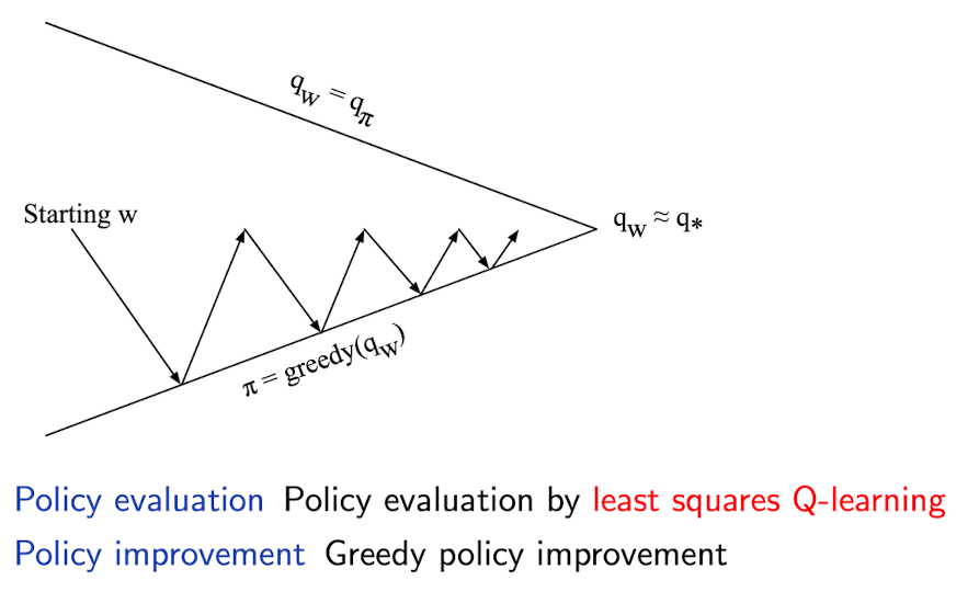
[Least Squares Policy Iteration(LSPI)]

[Least Squares Action-Value Function Approximation]
- Approximate action-value function $\color{blue}q_{\pi}(s,a)$ using linear combination of features $\mathrm{x}(s,a)$
$$\hat{q}(s,a,\mathrm{w}) = \mathrm{x}(s,a)^{\mathrm{T}} \approx q_{\pi}(s,a)$$
- Minimized least squares error between $\hat{q}(s,a,\mathrm{w})$ and $q_{\pi}(s,a)$
- from experience generated using policy $\pi$ consisting of $\left\langle \left( \text{state, action} \right),\text{value} \right\rangle$ pairs
$$\mathcal{D} = \left\{ \left\langle \left( s_{1}, a_{1} \right), v_{1}^{\pi} \right\rangle, \left\langle \left( s_{2}, a_{2} \right), v_{2}^{\pi} \right\rangle, \dots, \left\langle \left( s_{T}, a_{T} \right), v_{T}^{\pi} \right\rangle \right\}$$
[Least Squares Control]
For policy evaluation, we want to efficiently use all experience. For control, we also want to improve the policy. This experience is generated from many policies. So to evaluate $q_{\pi}(S,A)$ we must learn off-policy. We use the same idea as Q-learning:
- Use experience generated by old policy $S_{t}, A_{t}, R_{t+1}, S_{t+1} \sim \pi_{\text{old}}$
- Consider alternative successor action $A^{'} = \pi_{\text{new}}(S_{t+1})$
- Update $\hat{q}(S_{t},A_{t},\mathrm{w})$ towards value of alternative action $R_{t+1}+\gamma\hat{q}(S_{t+1},A^{'},\mathrm{w})$
*Least Squares Q-Learning
- Consider the following linear Q-learning update
$$\begin{array}{rcl}
\delta & =& R_{t+1}+\gamma\hat{q}(S_{t+1}, \color{red}\pi(S_{t+1})\color{black}, \mathrm{w})-\hat{q}(S_{t}, A_{t}, \mathrm{w}) \\
\Delta\mathrm{w} & = & \alpha\delta\mathrm{x} (S_{t}, A_{t})
\end{array}$$
- LSTDQ algorithm: solve for total update = zero
$$\begin{array}{rcl}
0 & = & \sum_{t=1}^{T}\alpha \left( R_{t+1}+\gamma\hat{q}(S_{t+1}, \color{red}\pi(S_{t+1})\color{black}, \mathrm{w})-\hat{q}(S_{t}, A_{t}, \mathrm{w}) \right)\mathrm{x}(S_{t},A_{t}) \\
\mathrm{w} & = & \left( \sum_{t=1}^{T}\mathrm{x}(S_{t},A_{t})(\mathrm{x}(S_{t},A_{t})-\gamma\mathrm{x}(S_{t+1},\pi(S_{t+1})))^{\mathrm{T}} \right)^{-1} \sum_{t=1}^{T}\mathrm{x}(S_{t},A_{t})R_{t+1}
\end{array}$$
*Least Squares Policy Iteration Algorithm
- The following pseudocode uses LSTDQ for policy evaluation
- It repeatedly re-evaluates experience $\mathcal{D}$ with different policies

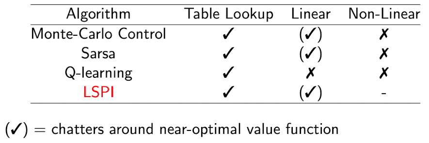
*Convergence of Control Algorithms

'Reinforcement Learning' 카테고리의 다른 글
| [RL] Introduction to Multi-Armed Bandits (1) (0) | 2023.06.26 |
|---|---|
| [RL] 7. Policy Gradient Methods (0) | 2023.05.04 |
| [RL] 5. Model-Free Control (2) | 2023.04.05 |
| [RL] 4. Model-Free Prediction (0) | 2023.03.29 |
| [RL] 3. Planning by Dynamic Programming (0) | 2023.03.07 |
